
Basics
Login & Analysis TypesPATENTS
Understand the Radar
Create an Analysis
Create a Dataset to Analyze
View Analysis
Find on Radar
DOCUMENTS
Understand the Radar
Upload data to Analyze
Create an Analysis
View Analysis
Find on Radar
SCOPE
Understand the Radar
Select Data Source
Create an Analysis
On the Radar
Find on Radar
User Guide.
PATENT Radar.
Understand the Radar
Patents in the data set are text mined and grouped together in clusters based on semantic similarities, or individual plots are created if an unclustered analysis is selected. Then they are run through multi-dimensional scaling and precisely positioned on a 2D radar based on their differences. Each dot represents one cluster or plot, with the size of the cluster reflecting the number of patents it contains. The closer the clusters the more similar their contents are. The XY axes have no particular meaning: distance is the focus of the data landscape.
Contour lines are created based on document density in areas of the radar, indicating possible semantic similarities or other levels of connectivity.
The analysis is automatically based on the company or organization that has the most patents in the data set: the Target Company. The others on the target list are the ones with the closest centers of gravity (overall document similarity) and filing ranges to the target company.
Get Started!
Create an Analysis
Select Patents → Patent Office → Start
NOTE
Patent OfficeJapan = JPO
United States = USPTO
Europe = EPO
WIPO = WIPO
Multiple = JPO Granted and Application, or USPTO and EP Granted and Application plus WIPO Application
NOTE
Select StatusApplication or Granted.
For WIPO, only Application is available
Create a Data Set to Analyze
Name: enter the name you'd like to give the data set.
Search type: select Text (concept search) or Patent Number.
Search query: enter up to 520K characters in the query box for a concept search, or enter patent numbers for the basis of the analysis. For best accuracy with text searches, the more words the better. If less than 5 are entered, any document containing any of the words can be included in the results (creating noise). Note that the tool mainly extracts and utilizes nouns, verbs, and adjectives for the analysis.
NOTE
For WIPO and EPO patent searches, the type of document must be included in the number, e.g. WO1991011363A1If patent numbers are entered in the query box, the text in the patent(s) will be mined and similar documents will be included in the results. To analyze a list of specific patents only, use the Upload Patent List File function (see below)

Advanced Options:
Part of Document to Search:
Full Text searches the entire document.
Abstract and Claims searches just that part of the document.
Full Text with emphasis on Abstract and Claims searches the entire document and puts extra weight (priority) on the Abstract and Claims.
Number of patents: enter the maximum number of patents you'd like to include in the data set, up to 100K.
Filter by Bibliographic Data:
NOTE: Using quotation marks when filtering helps reduce noise in the data set, e.g. "fuel cell" or "Apple, Inc". You can also use search operators AND, OR, (-) negation, ( ), and "string literal".
Title: use to search by words in a patent title.
Applicant: applicant/assignee refers to the company or organization name, e.g. Hitachi or Harvard University.
Latest Assignee: refers to the most recent owner of a patent. Only available on US-A, US-R, JP-A, and JP-R.
Inventor: full names must be input with last name, then a comma, then first name. e.g. EDISON, Thomas.
IPC: single IPCs must be entered as, e.g., B64C. If adding IPC classification group/subgroup, it must be in quotation marks with spacing between the code and number. Use two spaces if the group/subgroup has 4 digits, e.g., “B64C␣␣15/12”, and three spaces if the group/subgroup has 3 numbers, e.g. "B64C␣␣␣9/00". If doing multiple, follow the same spacing rules with AND or OR in between, e.g., “B64C 15/12” AND “B64C 9/00”.
Use only primary IPC: extracts only patents with the entered IPC if it is the primary (main) IPC.
Time range: enter the year range for the search (based on publication date).
Or Upload Patent List File: upload a .xlsx, .csv, .tsv, or .txt file of the patent numbers you'd like to analyze.
NOTE
Or Upload Patent List File: The list must contain patent numbers corresponding to the status (Application or Granted) and issuing authority (e.g. USPTO-A, EPO-G, etc.) of the selected database. [Download a sample] (US-R)Delete and change package: to stop this process and return to the home page, click [X] next to the current package. All data entered for this search will be erased.
Create Data Set: click to create the data set.
Data Sets: view all of your data sets here. To analyze, select one or multiple data sets you want to include in an analysis.

Under Analyze, confirm the Data settings:
Analysis Name: enter the name you'd like to give your analysis. If left blank, an analysis number will automatically be assigned.
Data Set: selected data sets will be listed here. Total Documents gives the cumulative number of patents in all selected data sets.
Part of Document to Analyze: confirm the part of the patent to be used for the analysis.
Sampling Threshold: confirm the number of patents to include in the analysis.
NOTE
If the total number of patents in the selected data sets is higher than the maximum allowable on your account, a calculated sampling will be extracted for the analysisUse Options to apply custom rules to the analysis calculation.
Name Normalization is the aggregation of IPC, company, or inventor names. To apply a new rule, create and upload a file under the More dropdown → Name Normalization. Sample File
Cluster Strength increases or decreases the cluster volume by adjusting the similarity threshold.
Strong → fewer clusters with more documents per cluster.
Weak → more clusters with fewer documents per cluster.
Cluster Count allows you to specify the exact number of clusters created during the calculation process. To create an unclustered analysis, enter the Total Documents number of the data sets you want to analyze. See Data → Data Set → Total Documents.
Word Importance is the adjustment of the level of relevance of certain words during the similarity calculation and clustering process. Words can be emphasized, weakened, or excluded. To apply a new rule, create and upload a file under the More dropdown → Word Importance. Sample File
Word Grouping puts synonymous words together and runs them as one in the calculation process. To apply a new rule, create and upload a file under the More dropdown → Word Grouping. Sample File
Indexical Analyzer controls the parameters of the 2D visualization according to the number of documents in the data set and the scope of their contents. If a data set broadly covers a topic or field, e.g. renewable energy, set it to broad. If it is specific, e.g. solar power energy storage and transfer, set it to specific. For patent volume, low is less than 10,000. Average is 10,000-50,000. High is 50,000+.
Advanced Options: adjust calculation settings for Contour Lines, Gravity Distance Transition, and Noteworthy Areas.

Click Run Analysis to start.
Your Analysis is in Progress: view the status of your analysis here. When complete, you will be notified by email. You can leave this page without affecting the progress. You can check the status under My Analyses.
NOTE
Depending on the document volume, it can take a few minutes to several hours to run the analysisAfter running an analysis, it will be listed on the Create/Analyses page under My Analyses, and on All Analyses from the More dropdown. You can hide, download, share, and delete analyses on this list.
View Analysis
Under My Analyses or from All Analyses, select the analysis you'd like to view.

1. Return to your list of analyses or create a new one
2. Manage your data sets
3. Manage your word importance, word grouping, and name normalization files, and view your browsing history and license usage, or access your All Analyses page
4. Adaptive list: click to view all visible documents on the radar
5. Full screen
6. Cluster size control
7. Zoom
Adaptive List: contains all clusters and patents in the analysis and is located beneath the radar. The list adjusts based on Quick Highlight and Filter selections to show only the clusters you have highlighted on the radar.

1. Create a new data set, create a sub-radar, or view all documents on the list
2. Order by cluster size (number of patents in the cluster)
3. Order by distance from the center of the radar
4. Pin the cluster on radar
5. Expand to show the full list of patents in the cluster
6. Number of patents in the cluster
Find on Radar
Analysis Information: view the metadata of the analysis, access contained data sets, and view statistical info of the analysis.
TARGET COMPANY is the basis for the SWOT analysis, Trend Graphs, Center of Gravity & Distribution Area, and Overview Graphs. Target company default is based on highest document volume, default Competitors List is based on closest proximity of center of gravity to the Target. Click the pop-out icon to change, add, or delete Target Company or Competitors.
SHARE, PRINT, +SUBSET are also accessed here.
Quick Highlight: highlight or isolate clusters based on keywords, years, assignees, inventors, or IPCs.
OR displays the clusters that contain the selected item/s. (Cluster-based search)
AND displays the clusters that contain ALL of the items selected. (Cluster-based search)
IN isolates clusters containing individual documents with all selected data-points. (Document-based search)
FILTER displays ONLY the selected items.
UPDATE CONTOUR adjust the contours based on what is visible on the radar when Filter is activated.
SCALE adjusts the cluster size based on relevant document ratio and pre-selects the data-points on the cluster page based on your selected items. Single click on the circle next to the selected items to change the highlight color.
SELECTED brings selected items to the top of the list.
CLEAR erases all selections on Quick Highlight and returns clusters to default.
Key Areas: highlight major (high density), growing, or sparse (low density surrounded by high density) areas on the radar.
NOTE
Key Areas labels are off by default. To activate them, go to Layers → Key Areas and select.For additional indicators, activate the Noteworthy Areas layer.
M: Major: in or near highest contour peaks, G: Growing: indicating faster growth than other regions, S: Sparse: indicating lower density within higher density regions, N: Newer: based on Cluster Trend, U: Unique: based on Density Graph, W: Weakness: based on SWOT, P: Strength: based on SWOT
Trend Graph: shows the target and its competitors’ centers of gravity movement over the time range of the data set. Click on a company to view its trend graph, and single click on the circle next to the company name to change the highlight color.
NOTE
You can add or remove companies on the list by accessing Analysis Information → Target CompanyCenter of Gravity and Distribution Area: shows the overlap and distances between the target's patent distribution range and center of gravity compared to others in the data set. Single click on the circle next to the selected companies to change the highlight color.
Cluster Trend: highlight the clusters containing the newest patents (based on issue date), largest number of patents, and closest to the centroid of the analysis. Click to highlight on the radar. Single click on the circle next to the cluster number to change the highlight color.
SWOT: view the target company’s strong and weak areas (based on relative document volume, growth rate, uniqueness, and filing trend compared to others in the data set), its nearest assignee (the one with the most overall similar documents) and its caution assignee (the one moving fastest towards its center of gravity). Click to highlight on the radar. Single click on the circle next to the cluster number to change the highlight color.
Overview Graphs:
Density: shows the integration density of each cluster of the target company. X and Y axes are the integration density of the target compared to others in the data set. The blue line is a least-squares method regression line. The red dotted lines are 3-sigma lines. The plots above the blue line are the target's strengths, those below are its weaknesses. The further from the axes origin the more unique. (See SWOT above for more details)
Gravity Distance Transition: shows the changes in distance between the target's center of gravity and the others', showing divergence or convergence trends over the time range of the data set. Target is represented by the X-axis.
Distance vs Trend: indicates the level of competitive caution of the target vs others. X and Y axes are the distance and trends between the target's center of gravity and the others' gravity. Positive and negative numbers indicate if their center of gravity is moving away from (+) or approaching (-) the target. Also see synergy classifications above.
Distance vs Radius of Area: shows the overlap and distances between the target's patent distribution range and center of gravity compared to others in the data set. X-axis shows the area of distribution. Y-axis shows the distance between the target's gravity and the others. Plots to the left of the green line indicate an overlap with the target, while to the right of the line indicates none. Also see synergy classifications above.
Number of Applicants in documents: indicates the number of documents an applicant has in the data set.
Number of Inventors in documents: indicates the number of documents that an inventor is connected to in the data set.
Number of documents in IPCs: indicates the number of documents containing a specific IPC.
Number of documents in Applicant: indicates the number of documents an applicant has over the time-period of the data set.
Number of documents in Inventor: indicates the number of documents that an inventor is connected to over the time-period of the data set.
Number of documents in IPCs: indicates the number of documents containing a specific IPC over the time-period of the data set.

Filters: create and manage customized filters.
Name: enter filter name (required).
Color: select color.
Border Width: set 0 for a cluster fill. Set 1-10 to circle the cluster. The higher the number the thicker the circle.
Shared Filter: set ON to make filter shareable across all analyses.
Document-based: Will highlight clusters containing individual documents that match all conditions.
Cluster-based: Will highlight clusters whose combined data satisfy all conditions.
To create a filter: select the filter target → select the target operator → enter the condition value.
To apply multiple conditions: Click the plus mark (+) to add a new condition, and click the minus (-) mark to remove a condition. There is no limit on the number of conditions.
When applying multiple conditions, they are calculated in the order they are entered. The calculation flow and an example of output is as follows:
Condition 1 and Condition 2 = Output A
Output A and Condition 3 = Output B
Output B or Condition 4 = Output C
Output C and Condition 5 = Output
Output D is what will be the final value of the filter.
In other words: (((1 and 2) and 3) or 4) and 5 = OutputSave: click save to create and apply the filter.
CONDITION OPTION - NOTES:
Data sets: enter the number located on the data set details pop-up on Data Sets page.
F-Terms: applicable only with Japanese patents
Cluster ID: enter a numerical value
Live or Die: terms for Application status:
Patent Office and Status values:
JP Application → jp
JP Granted → jppub
US Application → usapp
US Granted → usreg
EPO Application → epa
EPO Granted → epb
WIPO Application → woa
LIVE | DEAD |
| maintain | expired |
| non_payment | cancelled |
| rejected | withdrawn |
| applied | |
| deemed_maintain | UNKNOWN |
| deemed_exam | unknown |
NOTE
Live or Die filter options are not applicable on the Multiple and Japan Application + Granted packages.To view, edit, and delete shared filters, use Manage Shared Filters.
Areas: select and analyze areas on the radar.
Use Areas to select and view all documents in an area, create a new data set from documents in an area, or create a sub-radar based on the documents in an area.
Once an area is created, hover over the area and click Manage area to edit area information, create data set from area, create a sub-radar from documents in area, change the shape, angle, position of area, or delete area.

Contour Graph: shows the density of patents in areas of the radar.
Levels: sets the number of contour line intervals. The higher the number the sharper the contour regions.
Range: controls the displayed portion of Levels.
Factor: increases or decreases contour line detail in low density areas.
Create Areas from Lowest Contour Lines: shows keywords of lowest contour levels, and activates Areas functions.
Update the Contours Automatically: adjusts the contour regions automatically based on Highlight selections.
Heat Map: controls contrast of the radar based on contour regions.
Reset: returns the settings to the default.
NOTE
If the Contour Region has a square outline, it can be removed by lowering the Factor Level, or increasing the Contour Range Threshold in Advanced Settings - accessible through Radar Settings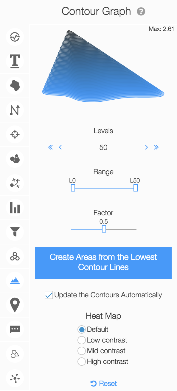
Text Plots: places an X on the radar to indicate the center of an area containing specified text. Enter single or multiple words in the search query and click save to mark the spot.
Pins: contains a list of pins you have placed on the radar.
Comments: contains a list of comments you have placed on the radar.
Drawing on Radar: draw and label areas on the radar.
Snapshot Mode: hide icons, metadata, and Target Company on the radar. Use your OS screenshot function to capture the radar.
Layers: control the visible layers on the radar.
DYNAMIC ACTIVATION enables layers to automatically come on when relevant functions are opened, even if they have been deselected on the Layers list. For example, the Clusters layer will automatically come on when the Quick Highlights function is opened.
Cluster Select: lists the cluster(s) you have clicked on the radar, including key words, years, and patents, and lists the history and access count of clusters you have clicked on the radar.
Radar Settings: control the settings of the radar.
RADAR SCALE adjusts the degree of zoom.
CLUSTER SIZE adjusts the size of the clusters.
BACKGROUND COLOR adjusts the background of the radar.
MAIN CLUSTER COLOR adjusts the default cluster color.
SHOW CLUSTER BORDER adds a thin border around all clusters.
CLUSTER POP-UP gives the option for hover-over or right-click pop-ups of cluster content on the radar.
ADVANCED OPTIONS allows adjustment of the advanced calculation and visualizations settings.
CLEAR ALL will remove selections on Quick Highlight, Trend Graph, Center of Gravity & Distribution Area, Cluster Trend, SWOT, Drawing on Radar, and custom zoom and cluster size will return to default. Areas, Filters, Pins, Comments, and Text Plots will not be removed.

Competitor List
Determines the companies that are considered possible competitors against the Target Company, and are listed on Trend Graph, Center of Gravity & Distribution Area, SWOT, and Overview Graph functions.
Select Based on Volume to have the list be based on companies with the highest document volumes.
Select Based on Proximity to have the list be based on companies with the nearest centers of gravity (the focal point of a company's core document area) to Target Company.
*The default Target Company is the company with the most documents in the dataset. The default Competitors List contains the top 20 possible competitors based on document volume. You can adjust the Target or Competitors on the Analysis Information tab.
Contour
Contour Splits: Adjust the XY splits to increase or decrease the steps of the contour regions. The higher the number the sharper the regions.
Contour Range Threshold: Determines the % of documents in the data set that will be incorporated into contour regions, based on distance from the center of the radar.
Coefficient of Attenuation Function: Determines the interval of the counter lines. The higher the number the closer the lines are drawn.
* Contour lines can also be controlled directly on the radar. See Find on Radar → Contour Graphs.
Noteworthy Selection (Majority)
Sets the amount of cluster labeled with M (majority) on the radar. Majority represents clusters in or near the highest points of contour regions. Default of 10 means a maximum of 10 clusters can be labeled as ‘Major’.
* To view the output, go to Find on Radar → Layers → Noteworthy Areas and make sure it is on
Noteworthy Selection (Uniqueness)
Sets the amount of clusters by ratio labeled with U (uniqueness) on the radar. Uniqueness represents clusters in outlying areas. Default of 10 means a maximum of 10 clusters can be labeled as ‘Unique’.
* To view the output, go to Find on Radar → Layers → Noteworthy Areas and make sure it is on
Noteworthy Selection (Sparse)
Sparse represents regions of relatively low density compared to the surrounding high density areas. Adjust the XY Sparse Splits to increase or decrease the size of the mesh in the background of the radar that will be used to calculate ‘Sparse’ regions. The lower the numbers the larger the sections of the mesh, meaning there is a higher chance something might be labeled as ‘Sparse’.
Set the Sparse Range Threshold to determine the ratio of documents in a section of the mesh that must be reached to make it eligible for ’sparse’. The lower the % the higher the chance something will be labeled as ’sparse’.
Noteworthy Selection (Newer)
Newer Target Date default is 1 year back from the date the analysis was created. Push the date back to increase the time range for ‘Newer’ regions, or bring it forward to decrease the time range.
Number of Selection in Newer sets the the amount of cluster by ratio labeled with N (newer) on the radar. Newer represents clusters containing the relative newest documents from the Newer Target Date. Default of 10 means a maximum of 10 clusters can be labeled as ‘Newer’.
* To view the output, go to Find on Radar → Cluster Trend → Newest
Noteworthy Selection (Growing)
Adjust the XY Growing Splits to increase or decrease the size of the mesh in the background of the radar that will be used to calculate ‘Growing’ regions. The lower the numbers the larger the sections of the mesh, meaning there is a higher chance something might be labeled as ‘Growing’.
Set the Growing Range Threshold to the % of documents in the data set from the centroid to be incorporated into the calculation for 'Growing'. The default 90% means the 91-100 percentile of documents furthest from the center of the radar will not be included in the calculation.
Set the Growing Threshold Date to the starting point of the period of interest. Default is 5 years back from the date the analysis was created. Push the date back to increase the time range for ‘Growing’ regions, or bring it forward to decrease the time range. If you are working with a short time range, you should adjust appropriately.
Number of Selection in Growing sets the the amount of cluster by ratio labeled with G (growing) on the radar. Growing represents clusters with the fastest relative increase in documents from the Growing Threshold Date. Default of 10 means a maximum of 10 regions can be labeled as ‘Growing’.
Gravity Distance Transition
Select to calculate and display the overall gravity trend on the Gravity Distance Transition Graph.
* To view the output, go to Find on Radar → Overview Graphs → Gravity Distance Transition Graph
If you cannot find your answers here, send us a message. Potentially found a bug? Let us know!